Introduction to ggplot2

class: center, middle, inverse, title-slide

# Introduction to ggplot2
## Advanced plotting in R 2021
### Michael Matiu
### 2021/05/11

---

## Content

.pull-left[

### Block 1 (Intro and EDA)

- Fundamentals of ggplot2
    + Data
    + Language
- Building blocks
    + Mapping
    + Layering
    + Facetting
- ggplot2 for EDA (exploratory data analysis)
- some other gg packages

**HANDS ON DATA**

]

.pull-right[

### Block 2 (publication-ready plots)

- Basics of design
- Styling of ggplots
- Arranging multiple ggplots
- Annotating
- Polishing

**HANDS ON DATA**
]

---

## What is ggplot2?

Declarative plotting system built around the [Grammar of Graphics](https://www.amazon.com/Grammar-Graphics-Statistics-Computing/dp/0387245448/ref=sr_1_1?dchild=1&keywords=the+grammar+of+graphics&qid=1620283819&sr=8-1).

Created by Hadley Wickham some 10 years ago.

Declarative means: You need to define links to data, and ggplot will take care of the rest (axes, limits, scales, colours, labels, legends, ...).

---

## Why ggplot2?

Good:
+ easy to explore different visualizations
+ sensible default scales (x, y, colour, ...)
+ automatic legends
+ allows fast data exploration of multi-dimensional data by using different aesthetics (position, colour, shape, size, ...) and facetting
+ all-in-one-solution: good for both EDA (exploratory data analysis) and publication-ready figures

Bad:
- fine-tuning can be tedious
- sometimes, if you want to override ggplot2 defaults, it can be hacky or impossible

---

## Tidy data

ggplot2 is built around **tidy** data sets (data.frame, tibble, data.table).

.tiny[R4DS, https://r4ds.had.co.nz/tidy-data.html#tidy-data-1]

---

## Data wrangling: Observations in columns

```r
table4 %>% 
  pivot_longer(c(`1999`, `2000`), names_to = "year", values_to = "cases")
```

.tiny[R4DS, https://r4ds.had.co.nz/tidy-data.html#longer]

---

## Data wrangling: Observations scattered across rows

```r
table2 %>% 
  pivot_wider(names_from = key, values_from = value)
```

.tiny[R4DS, https://r4ds.had.co.nz/tidy-data.html#wider]

---

## Data wrangling: Transformation

```r
# select observations
flights %>% 
  filter(month == 1, day == 1)

# create new columns
flights %>% 
  mutate(gain = dep_delay - arr_delay,
         speed = distance / air_time * 60)

# summarize by groups
flights %>% 
  group_by(year, month, day) %>% 
  summarise(delay = mean(dep_delay, na.rm = TRUE))
```

---

## ggplot2 components and language

#### Minimally required

- A default dataset 
- Set of mappings from variables to aesthetics
- One or more layers, each composed of 
    + a geometric object

#### Optional (to override defaults)

- For each layer
    + a statistical transformation
    + a position adjustment
    + optionally, different dataset and aesthetic mappings
- One scale for each aesthetic mapping
- A coordinate system
- The faceting specification

---

## Aesthetics

Describe graphical elements

Continuous vs. discrete

.tiny[Source: Claus O. Wilke, *Fundamentals of Data Visualization*, https://clauswilke.com/dataviz/aesthetic-mapping.html]

---

## Scales

Map data values onto aesthetics

.tiny[Source: Claus O. Wilke, *Fundamentals of Data Visualization*, https://clauswilke.com/dataviz/aesthetic-mapping.html#scales-map-data-values-onto-aesthetics]

---

## Geoms - Basic building blocks

.tiny[Source: Hadley Wickham, *ggplot2 book*, https://ggplot2-book.org/individual-geoms.html]

---

## Code structure

```r
ggplot(data = <DATA>)+ # REQUIRED
  <GEOM_FUNCTION>(mapping = aes(<MAPPINGS>), # REQUIRED
                  stat = <STAT>, position = <POSITION>)+ # optional
  <COORDINATE_FUNCTION>+ # optional
  <FACET_FUNCTION>+ # optional
  <SCALE_FUNCTION>+ # optional
  <THEME_FUNCTION> # optional
```

---

## Layering

.panelset[
.panel[.panel-name[Base]

.pull-left[

```r
*ggplot(mpg, aes(displ, hwy))
```

]

.pull-right[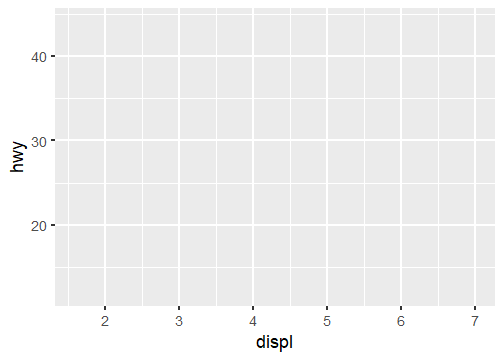

![](ggplot-01-intro_files/figure-html/unnamed-chunk-6-1.png)

]

.panel[.panel-name[1 geom]
.pull-left[

```r
ggplot(mpg, aes(displ, hwy))+
* geom_point()
```

]

.pull-right[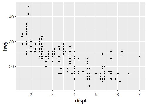
![](ggplot-01-intro_files/figure-html/unnamed-chunk-8-1.png)
]
]

.panel[.panel-name[2 geoms]
.pull-left[

```r
ggplot(mpg, aes(displ, hwy))+
  geom_point()+
* geom_smooth()
```

]
.pull-right[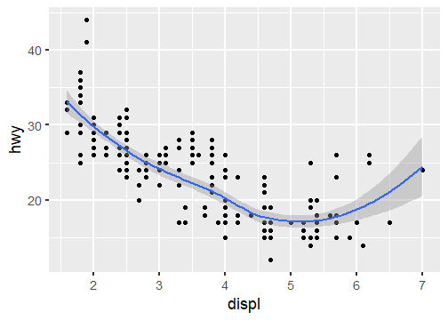
![](ggplot-01-intro_files/figure-html/unnamed-chunk-10-1.png)
]
]

.panel[.panel-name[3 geoms]
.pull-left[

```r
ggplot(mpg, aes(displ, hwy))+
  geom_point()+
  geom_smooth()+
* geom_hline(yintercept = 30, linetype = "dashed")
```

]
.pull-right[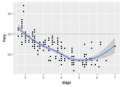
![](ggplot-01-intro_files/figure-html/unnamed-chunk-12-1.png)
]
]

]

---

## Inheritance of aes()

All of these produce the same plot:

```r
ggplot(mpg, aes(displ, hwy, colour = class)) + 
  geom_point()

ggplot(mpg, aes(displ, hwy)) + 
  geom_point(aes(colour = class))

ggplot(mpg, aes(displ)) + 
  geom_point(aes(y = hwy, colour = class))

ggplot(mpg) + 
  geom_point(aes(displ, hwy, colour = class))
```

Within each layer you can add, override, or remove (set to `NULL`).

---

## Setting vs. mapping of aesthetics

.panelset[

.panel[.panel-name[Mapping]
.pull-left[

Within `aes()` the aesthetic is mapped to a variable.

```r
ggplot(mpg, aes(displ, hwy))+
* geom_point(aes(colour = drv))
```

]

.pull-right[
![](ggplot-01-intro_files/figure-html/unnamed-chunk-15-1.png)
]
]

.panel[.panel-name[Setting]
.pull-left[

Outside `aes()` the aesthetic is set to a value. Needs to be a possible value then.

```r
ggplot(mpg, aes(displ, hwy))+
* geom_point(colour = "darkblue")
```

]

.pull-right[
![](ggplot-01-intro_files/figure-html/unnamed-chunk-17-1.png)
]
]

.panel[.panel-name[Setting in aes()]
.pull-left[

What happens, if we set a value within `aes()`?

```r
ggplot(mpg, aes(displ, hwy))+
* geom_point(aes(colour = "darkblue"))
```

]

.pull-right[
![](ggplot-01-intro_files/figure-html/unnamed-chunk-19-1.png)
]
]

.panel[.panel-name[Mapping constants]
.pull-left[

One can also "manually" construct mappings. Can be useful in certain cases.

```r
ggplot(mpg, aes(displ, hwy)) + 
  geom_point() +
* geom_smooth(aes(colour = "loess"),
              method = "loess", 
              se = FALSE) + 
* geom_smooth(aes(colour = "lm"),
              method = "lm", 
              se = FALSE)
```

]

.pull-right[
![](ggplot-01-intro_files/figure-html/unnamed-chunk-21-1.png)
]
]

]

---

## Coordinate systems

Not that relevant, since mostly the Cartesian one is used.

However you can force a fixed aspect ratios `coord_fixed()` or use polar coordinates `coord_polar()`.

This flexibility allows easy extension: `coord_sf()` for spatial data (`->` Mattia).

---

## Facetting - Basics

Generate small multiples based on subsets of the data.

Incredibly powerful technique.

ggplot offers two different options:

.tiny[Source: ggplot2 book, https://ggplot2-book.org/facet.html]

---

## facet_wrap

.panelset[
.panel[.panel-name[base]
.pull-left[

```r
# some random data
n_grp <- 8
n_points <- 10

tbl_wrap <- tibble(
  grp = rep(LETTERS[1:n_grp], each = n_points),
  xx = rep(1:n_grp, each = n_points) + 
    rnorm(n_grp*n_points),
  yy = rep(n_grp:1, each = n_points) + 
    rnorm(n_grp*n_points)
)
```

```r
# wrap grp
ggplot(tbl_wrap, aes(xx, yy))+
  geom_point()+
* facet_wrap(~grp)
```

]

.pull-right[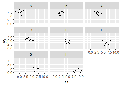
![](ggplot-01-intro_files/figure-html/unnamed-chunk-24-1.png)
]
]

.panel[.panel-name[free scales]
.pull-left[

```r
ggplot(tbl_wrap, aes(xx, yy))+
  geom_point()+
* facet_wrap(~grp, scales = "free")
```

Also possible to use `"free_x"` or `"free_y"`.

]

.pull-right[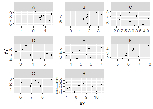
![](ggplot-01-intro_files/figure-html/unnamed-chunk-26-1.png)
]
]

.panel[.panel-name[nrow ncol]
.pull-left[

```r
ggplot(tbl_wrap, aes(xx, yy))+
  geom_point()+
* facet_wrap(~grp, nrow = 2)
```

Also possible to specify number of columns with `ncol = `.

]

.pull-right[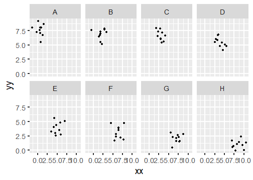
![](ggplot-01-intro_files/figure-html/unnamed-chunk-28-1.png)
]
]

.panel[.panel-name[Order of wrapping]
.pull-left[

```r
ggplot(tbl_wrap, aes(xx, yy))+
  geom_point()+
* facet_wrap(~grp, nrow = 2, dir = "v")
```

Standard is `dir = "h"`.

]

.pull-right[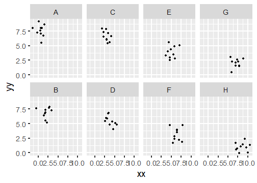
![](ggplot-01-intro_files/figure-html/unnamed-chunk-30-1.png)
]
]

.panel[.panel-name[Order of elements]
.pull-left[

The order of facets is determined by the underlying factor. If it's a character vector, then alphabetically. In order to change the order, you need to modify the factor.

```r
tbl_wrap %>% 
  mutate(grp_f = fct_relevel(factor(grp),
                             "B", "G", "E", "F", 
                             "D", "A", "C", "H")) %>%
  
  ggplot(aes(xx, yy))+
  geom_point()+
  facet_wrap(~grp_f, nrow = 2)
```

]

.pull-right[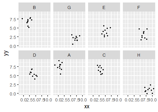
![](ggplot-01-intro_files/figure-html/unnamed-chunk-32-1.png)
]
]

]

---

## facet_grid

.panelset[
.panel[.panel-name[x ~ .]
.pull-left[

```r
# some random data
n_points <- 10
tbl_grid <- tibble(
  grp1 = rep(c("A", "B", "C"), each = n_points*3),
  grp2 = rep(rep(c("X", "Y", "Z"), n_points), 3),
  xx = rep(1:9, each = n_points) + rnorm(9*n_points),
  yy = rep(9:1, each = n_points) + rnorm(9*n_points)
)
```

```r
# plot
ggplot(tbl_grid, aes(xx, yy))+
  geom_point()+
* facet_grid(grp1 ~ .)
```

]

.pull-right[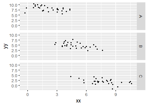
![](ggplot-01-intro_files/figure-html/unnamed-chunk-35-1.png)
]
]

.panel[.panel-name[. ~ y]
.pull-left[

```r
ggplot(tbl_grid, aes(xx, yy))+
  geom_point()+
* facet_grid(. ~ grp2)
```

]

.pull-right[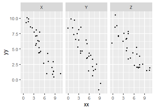
![](ggplot-01-intro_files/figure-html/unnamed-chunk-37-1.png)
]
]

.panel[.panel-name[x ~ y]
.pull-left[

```r
ggplot(tbl_grid, aes(xx, yy))+
  geom_point()+
* facet_grid(grp1 ~ grp2)
```

]

.pull-right[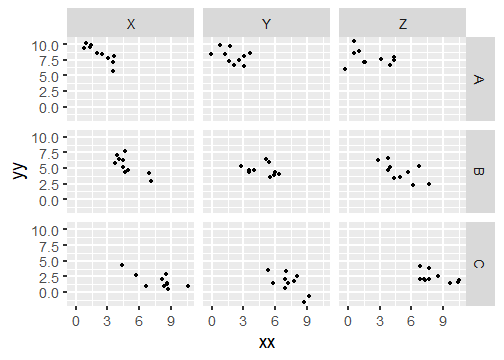
![](ggplot-01-intro_files/figure-html/unnamed-chunk-39-1.png)
]
]

.panel[.panel-name[free space]
.pull-left[

Besides free scales, for `facet_grid` you also have `space =`. So height/width is proportional to range of data.

```r
tbl_grid %>% 
  mutate(yy_shrink = if_else(grp1 == "B", 
                             (yy - mean(yy))/sd(yy), 
                             yy)) %>% 
  
  ggplot(aes(xx, yy_shrink))+
  geom_point()+
  facet_grid(grp1 ~ grp2, 
             scales = "free", 
*            space = "free")
```

]

.pull-right[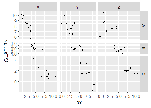
![](ggplot-01-intro_files/figure-html/unnamed-chunk-41-1.png)
]
]

.panel[.panel-name[free space 2]
.pull-left[

This is especially useful for categorical scales.

See example on the right from

https://ggplot2-book.org/facet.html#controlling-scales

]

.pull-right[
<img width=70% height=70% src="https://ggplot2-book.org/facet_files/figure-html/discrete-free-1.png">
]
]

]

---

## facets with continuous variables

If you want to facet on continuous variables, you need first to discretise it.

ggplot offers three helper functions:

- `cut_width(x, w)` <br> makes bins of the same width `w`
- `cut_interval(x, n)` <br> makes `n` bins of equal width
- `cut_number(x, n)` <br> makes `n` bins that approximately contain the same number of observations (with varying width)

Or you can use the base `cut()` function, which also allows you manually specify the breaks and labels.

---

## Grouping vs. facetting

.panelset[
.panel[.panel-name[Question]

Should you use groups (e.g. colour) or facets?

The answer is both.

And ggplot makes it easy to switch and try out all the options.

]

.panel[.panel-name[groups]
.pull-left[

```r
ggplot(tbl_grid, aes(xx, yy, colour = grp2))+
  geom_point()
```

]

.pull-right[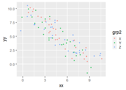
![](ggplot-01-intro_files/figure-html/unnamed-chunk-43-1.png)
]
]

.panel[.panel-name[facets]
.pull-left[

```r
ggplot(tbl_grid, aes(xx, yy))+
  geom_point()+
  facet_grid(. ~ grp2)
```

]

.pull-right[
![](ggplot-01-intro_files/figure-html/unnamed-chunk-45-1.png)
]
]

.panel[.panel-name[both]
.pull-left[

```r
ggplot(tbl_grid, aes(xx, yy, colour = grp1))+
  geom_point()+
  facet_grid(. ~ grp2)
```

]

.pull-right[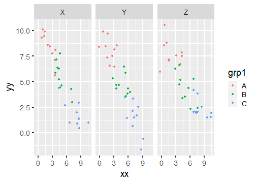
![](ggplot-01-intro_files/figure-html/unnamed-chunk-47-1.png)
]
]

]

---

## saving plots

.panelset[
.panel[.panel-name[as R objects]

You can save the call to `ggplot()+...` as R object.

```r
*gg <- ggplot(tbl_wrap, aes(xx, yy))+
  geom_point()+
  facet_wrap(~grp)
```

Some people use this to construct a plot sequentially.

```r
gg <- ggplot(tbl_wrap, aes(xx, yy))
gg <- gg + geom_point()
gg <- gg + facet_wrap(~grp)
```

]

.panel[.panel-name[as files]

```r
ggsave(
  filename = "abc.pdf", 
  plot = gg,
  width = 6,
  height = 4
)
```

- if you omit the `plot = ` argument, then the last plot is saved
- based on the ending of the filename, ggplot will choose the right device and sage the appropriate file, including PDF, PNG, JPG, TIFF, ...
- width and height are by default given in inches, but can choose cm or mm with the `units=` argument, e.g. `units = "cm"`
- tip to determine the plot size: plot it in the RStudio plots pane, use the "Export" button with "Save as PDF", use the "Preview" button, and play around with sizes

]

---

## ggplot for EDA

.panelset[
.panel[.panel-name[Why?]

The ggplot grammar makes it easy to try out and switch between many plots.

- explore many geoms
- exchange aesthetics
- use facets
- exchange facets with aesthetics

]

.panel[.panel-name[facet more variables]
.pull-left[

Using `+` you can add multiple groups to facet over

```r
ggplot(tbl_grid, aes(xx, yy))+
  geom_point()+
* facet_wrap(~ grp1 + grp2)
```

]

.pull-right[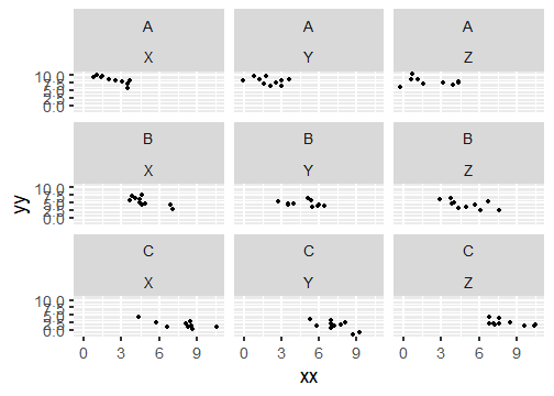
![](ggplot-01-intro_files/figure-html/unnamed-chunk-52-1.png)
]
]

.panel[.panel-name[loop and save]

```r
# get limits
xl <- range(tbl_wrap$xx)
yl <- range(tbl_wrap$yy)

# open pdf file (graphics device)
pdf("gg-loop.pdf", width = 6, height = 4)

# loop through all
for(i_grp in sort(unique(tbl_wrap$grp))){
  
  gg <- tbl_wrap %>% 
    filter(grp == i_grp) %>% # filter to grp
    
    ggplot(aes(xx, yy))+
    geom_point()+
    xlim(xl)+ # enforce same limits
    ylim(yl)+
    ggtitle(paste0("Group: ", i_grp)) # add some info
  
  print(gg) # inside for() loop needs a print() of the gg object
  
}
# close the pdf (device)
dev.off()
```

]

---

## some additional packages

`->` external file

---

## Now it's your turn!

.pull-left[

### A) Structured exercises

Go to the folder

`02_Ggplot/exercises/`

and start hacking!

Solutions will be provided after the end of the day.

]

.pull-right[

### B) Freely explore data

If you brought own data: Use it!

Otherwise, feel free to use the provided data in `00_Data/`. Consult the `Readme.md` inside for more info.

Explore, find patterns, try to answer question you have on the data, ...

]